I promised more examples of using monads to draw fractals. Let’s do some!

Today I’ll explain a simple method to draw lots of fractal pictures with minimal code, using the idea of Kleisli powers I introduced in the previous part. This will be easy to implement in Haskell, and accessible even if you’re not a Haskell programmer.
To do this, I’ll first introduce another well known way of drawing fractal pictures, using random motion. If you haven’t seen this before, it’s cool in its own right, but then we’ll change the rules slightly and generate fractals instead using monads. I’ll again be using the power set and list monads this time, so if you’ve read the first two parts, this should be familiar.
The Chaos Game
In the “Chaos Game” you pick a fixed set of affine transformations of the plane, usually all contraction mappings, and then watch what happens to a single point in the plane when you apply a randomly chosen sequence from our set of transformations.
For example, in the best-known version of this game we take just three transformations, each a scaling of the plane by a factor of 1/2, but each around a different fixed point. More precisely, fix points A, B, and C, the vertices of a triangle, and define three corresponding transformations  by
by

Here’s how the game typically starts:

I’ve picked a random starting point and a random sequence which begins B, A, C, B, B, B, A, A, B, … . You can see that at each step, we’re moving in a straight line half way to the next point in the sequence.
At first, it doesn’t sound doesn’t seem like anything very exciting is happening. But if we keep going, we find something interesting. To show the pattern more clearly, I’ll stop drawing the lines between steps, and just keep track of the successive points. I’ll also shrink the dots a little, to avoid them running into each other. Here’s what a typical random orbit looks like after 3000 iterations:

A picture of the Sierpinski triangle is already emerging. After 10,000 iterations it looks like this:
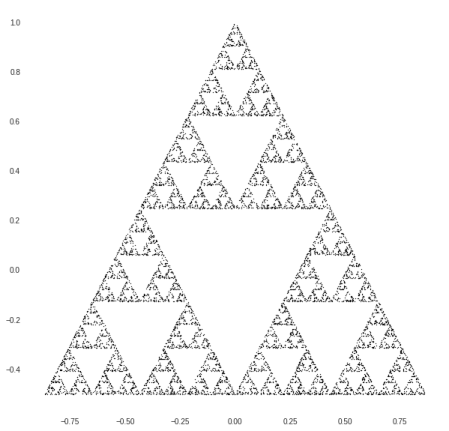
And after 50,000 iterations it’s getting quite clear:
There are tons of variations of the “chaos game,” which also go by the less flashy but more descriptive name of “Iterated Function Systems.” But let’s get to the monads.
Removing the Randomness with Monads
What does the Chaos Game have to do with monads? While it’s fun to generate fractal pictures using random motion, we can also trade this random process for a completely deterministic one in which we iterate a single morphism in the Kleisli category of a monad.
In general, an alternative to making random selections between equally likely steps is to take all of the possible steps simultaneously. That is, we can get rid of the randomness at the cost of replacing the ordinary functions  with a multi-valued function. Monads give us a nice way to handle this: we’ve seen before that multi-valued functions are just morphisms in the Kleisli category of the power set monad, and we can compose them using Kleisli composition.
In our case, the functions used in the chaos game are , which move points closer to A, B, C, respectively. We can combine these into a single function

given by

We then have only to iterate this.
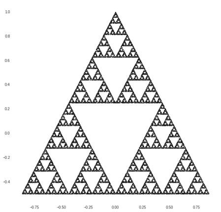
The resulting code gives us pictures similar to the ones for the original chaos game, but much more regular and symmetric, since we’ve avoided making any random choices by making all possible choices. If we also start out in a symmetric state, picking (0,0) as our starting point, and letting the fixed points A, B, and C form an equilateral triangle centered around this point, then at each generation thereafter we get a picture that has all of the symmetries of a triangle.
Here’s generation 6, with  points:

Here’s generation 8, with  points:

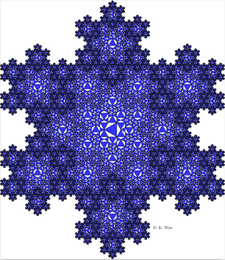
And here’s generation 10, with  points:

Comparing this to the picture from the chaos game with 50,0000 iterations, the two are very similar, though the “monadic” version has sharper edges, and none of the small scale noise of the random version.
The code
To implement this in Haskell, I need to define what a point in the plane is, and define a few operations on points. I’ll define a new data type, Point, which really just consists of pairs of real (or more accurately, floating point) numbers, and I’ll define vector addition and scalar multiplication on these in the obvious way:
type Point = (Float,Float)

add :: Point -> Point -> Point
add (x1,y1) (x2,y2) = (x1+x2,y1+y2)

mult :: Float -> Point -> Point
mult r (x,y) = (r*x,r*y)
Sure, I could use a linear algebra library instead; I’m implementing these operations myself mainly because it’s easy, and perhaps more friendly and instructive for those new to Haskell.
Using these operations, we can build a function that scales the plane around a given point. I’ll do this more generally than in the examples above, because it will be useful for other versions of the chaos game which I’ll discuss later. If  is a point in the plane, and
  is a real number, then the function
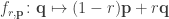
scales  by a factor around the point
  . Here’s a Haskell implementation of this function:
scaleAround :: Float -> Point -> Point -> Point
scaleAround r p q = ((1-r) `mult` p) `add` (r `mult` q)
This can be read as saying we take two parameters, a real number r and a point p, and this results in a function from points to points, which is really just  . The
. The ` marks around add and mult let us use these as “infix” operators, as opposed to prefix operators like in Polish notation; for example 3 `mult` (1,0) means the same as mult 3 (1,0), and both give the result (3,0).
Now, we can make a list-valued function that will generate the Sierpinski triangle. First, let’s fix the vertices of our triangle, which will just be a list of Points:
triVertices = [(sin(2*k*pi/3), cos(2*k*pi/3)) | k <- [0..2]]
This is so much like the mathematical notation for sets that it needs no explanation; just squint until the <- starts to look like  , and remember that we’re dealing with Haskell lists here rather than sets.
As before, our function for generating this fractal combines all of the  where ranges over the vertices in the triangle:
f :: Point -> [Point]
f q = [scaleAround 1/2 p q | p <- triVertices]
The first line is the type signature of the function; it just says f takes a point as input, and returns a list of points as output. This is our morphism in the Kleisli category of the list monad. The rest of the code just amounts to taking Kleisli powers of this morphism. Recall that code from last time:
kpow :: Monad m => Int -> (a -> m a) -> a -> m a
kpow 0 _ = return
kpow n f = f <=< kpow (n-1) f
That’s everything we need. Let’s pick our starting point in  to be the origin, set the number of generations to 10, and calculate the output data:
startPt = (0,0) :: Point
nGens = 10

outputData = kpow nGens f $ startPt
The last line here takes the 10th Kleisli power of f, and then applies that to the starting point (0,0). The result is the list of points, and if you plot those points, you get the picture I already posted above:
More examples
Once you know the trick, you can build new versions of the chaos game to generate other fractals.
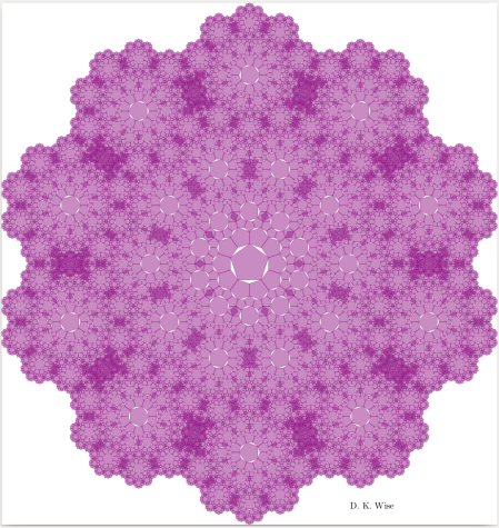
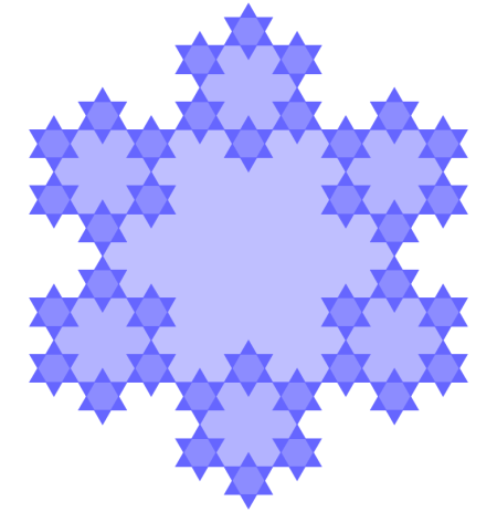
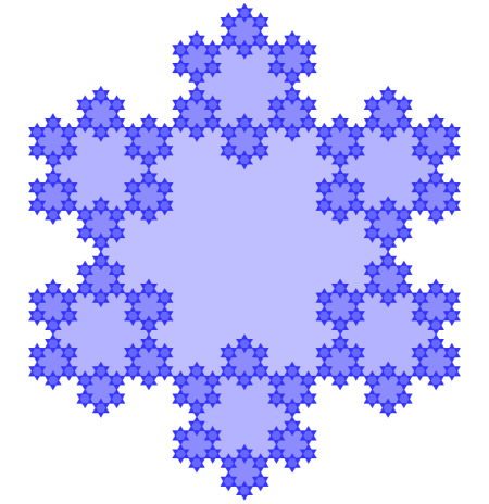
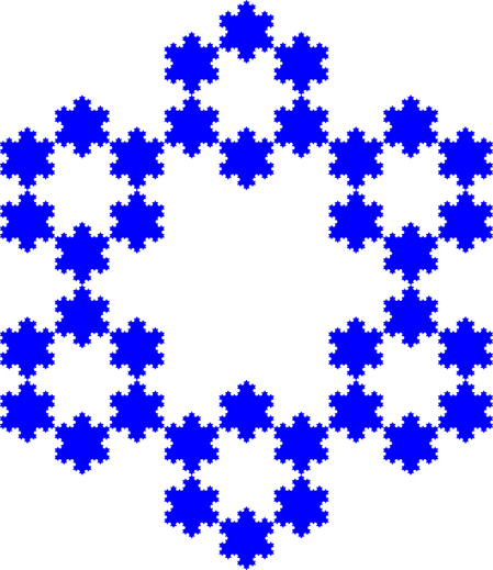
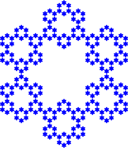
Here’s a fun one. Before, we started with an equilateral triangle and scaled around each of its vertices by a factor of 1/2; Now let’s take a regular hexagon and scale around each of its vertices by a factor of 1/3.
To build this using our monadic methods, all we really need to change in the code I’ve written above is which vertices and scaling factor we’re using:
hexVertices = [(sin(2*k*pi/6), cos(2*k*pi/6)) | k <- [0..5]]

f q = [scaleAround 1/3 p q | p <- hexVertices]
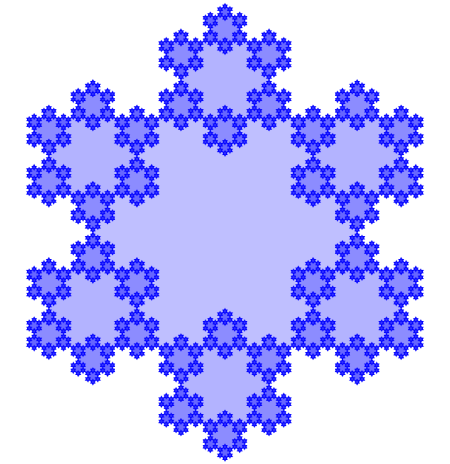
The result?

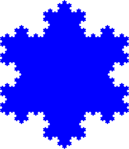
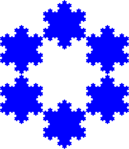
It’s a Koch curve! Or rather, it’s lots of copies of the Koch curve at ever smaller scales. This is just the fractal that I’ve written about before, starting with “Fun with the Koch Snowflake” which I wrote when I first discovered it. It’s like a “Sierpinski Koch snowflake” because it can also be built by starting with a Koch snowflake and the repeatedly removing a Koch snowflake from the middle to leave six new Koch snowflakes behind.
The reason this slightly modified chaos game gives the Sierpinski Koch snowflake is essentially that, at each stage, the Koch snowflake splits into six new Koch snowflakes, each a third of the size of the original, and distributed in a hexagonal pattern.
How does this generalize? There’s a whole family of fractals like this, which I posted about before, and there’s a version of the chaos game for each one.
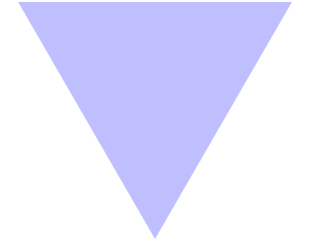
I explained in Fun with the Koch snowflake how this replication rule for triangles:

leads to the Sierpinski Koch Snowflake we found above:

Similarly, I explained how this replication rule for squares:

leads to an analogous fractal with octagonal symmetry:

and how this replication rule for pentagons:
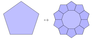
leads to this:

fractal with decagonal symmetry. This sequence continues.
To get the transformations needed for the chaos game, we just need to calculate how much smaller the polygons get in each successive generation. If you stare at the replication rules above, you can see that pattern I’m using: the edge of the parent polygon is congruent to two edges of the child polygon plus a segment extending from one vertex to the next-to-adjacent vertex of the child polygon. Solving this, the correct scaling factor is
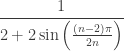 .
.
The chaos game—and the tamer “monadic” variant on it—for these fractals just amounts to scaling by this factor around each of the vertices in a regular  -gon.
-gon.
By the way, you might be tempted (I was!) to include some rotations in addition to the scale transformations, since in the polygon-based versions, only half of the polygons have the same angular orientation as their parent. However, these rotations turn out not to matter when we’re using points as our basic geometric objects rather than polygons.
Again, there’s little code we need to modify. First, since we need polygons with any number of sides, let’s make a function that takes an integer and gives us that many vertices distributed around the unit circle, with the first vertex always at 12 O’Clock:
polyVertices :: Int -> [Point]
polyVertices n = [(sin(2*k*pi/nn), cos(2*k*pi/nn)) | k <- [0..(nn-1)]]
    where nn = fromIntegral n
If you’re new to Haskell, this should all be familiar by now, except perhaps the last line. Haskell will complain if you try dividing a floating point number by an integer since the types don’t match, so the integer n has to be converted to a float nn; this makes k also a float, since the notation [0..x] actually means the list of all of the floating point integers from 0 to x, if x is a floating point number, and then everything in sight is a float, so the compiler is happy.
We then have to change our generating morphism to:
f :: Int -> Point -> [Point]
f n q = [scaleAround r p q | p <- polyVertices (2*n)]
    where r = 1/(2 + 2*sin((nn-2)*pi/(2*nn)))
          nn = fromIntegral n
and remember that the generating morphism is now not just f but f n.
Now we can set the starting point, the number of “sides” of the basic polygon, and the number of generations, as we wish:
startPt = (0.2,0.5) :: Point
m = 5               -- number of generations
n = 7               -- number of "sides"

outputData = kpow m (f n) $ startPt
Just remember that the final list is a list of  points, so don’t blame me if you make these numbers big and run out of memory. :-)
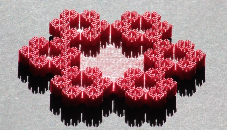
In any case, with code like this, you can generate analogs of the Sierpinski Koch snowflake based on squares:
Pentagons, which start “overlapping”:

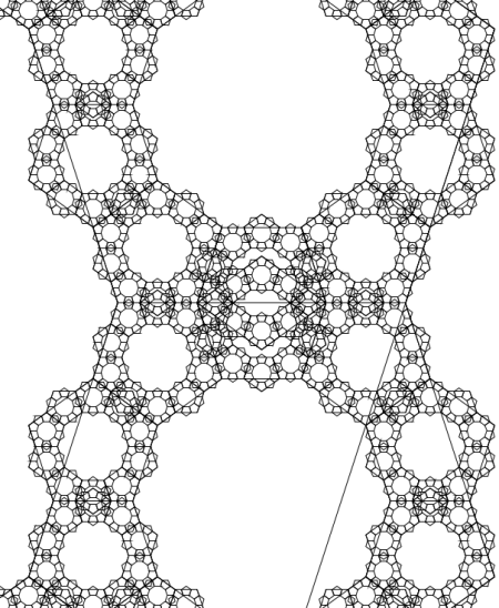
Hexagons, where the overlapping becomes perfect:

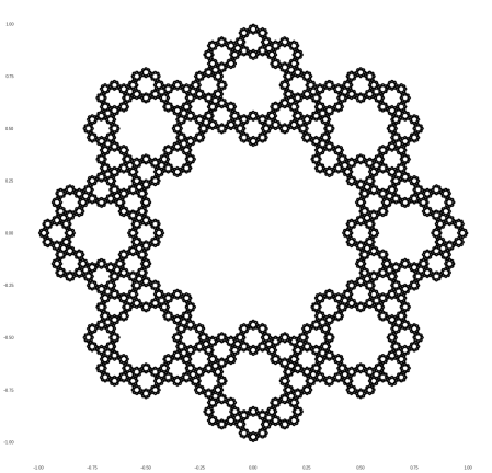
and more. Heptagons, where the overlapping gets a bit more severe:

Octagons:
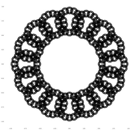
and so on.
But enough of that. Next time, I’ll move on to fractals of a different sort …


 . As an example, we had considered a map that takes any triangle in the plane to sets of three new triangles as shown here:
 leads us directly to the “Kleisli category” associated to the power set monad. I want to explain this here, because in computer science people actually tend to think of monads essentially in terms of their associated Kleisi categories, and that’s how monads are implemented in Haskell.
 in the category of sets, I’ll start with that special case.
 , the objects are the same as the original category
  : they’re just sets. A morphism from the set
  , however, is a function
 in the category
  as decoration on the arrow , rather than on the codomain object
  and
and  , the Kleisli composite
  is defined by
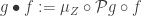
 in the Kleisli category:
 is associative, and that the maps
  are identity morphisms, so we really do get a category. That’s all there is to the Kleisli category.
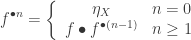
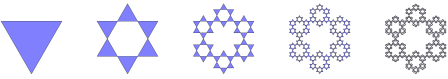
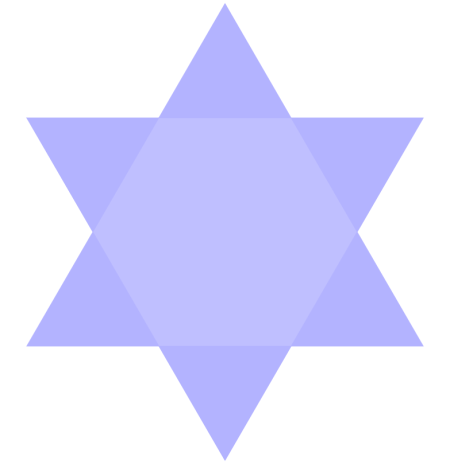
 of all equilateral triangles in the plane and consider the map
  defined so that
  has six elements, each 1/3 the size of, and linked together around the boundary of the original triangle
  , as shown here:
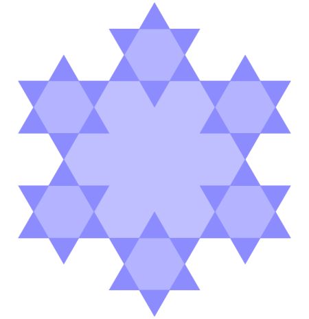
 the images under successive Kleisli powers of the generating endomorphism:
 , (i.e. something of type
 is any monad, and
  is any type. We take an integer and a Kleisli endomorphism for the monad m, and return another endomorphism. Notice there’s a slight discrepancy here, in that an
  . But the integer really is intended to be non-negative. If you fed a negative integer into
  for any object
  “, where the objects in this case are always data types.
 is written
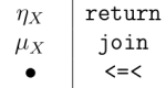
 , a.k.a.
 ![[x_1, x_2, \ldots x_n] \quad \text{where } x_i\in a](https://s0.wp.com/latex.php?latex=%5Bx_1%2C+x_2%2C+%5Cldots+x_n%5D+%5Cquad+%5Ctext%7Bwhere+%7D+x_i%5Cin+a&bg=ffffff&fg=333333&s=0&c=20201002)
![[x_1, x_2, \ldots]](https://s0.wp.com/latex.php?latex=%5Bx_1%2C+x_2%2C+%5Cldots%5D&bg=ffffff&fg=333333&s=0&c=20201002) for an infinite list.
for an infinite list. we get a function that just acts element-wise on lists:
![([x_1,x_2,\ldots, x_n]) \mapsto [f(x_1),f(x_2), \ldots f(x_n)]](https://s0.wp.com/latex.php?latex=%28%5Bx_1%2Cx_2%2C%5Cldots%2C+x_n%5D%29+%5Cmapsto+%5Bf%28x_1%29%2Cf%28x_2%29%2C+%5Cldots+f%28x_n%29%5D&bg=ffffff&fg=333333&s=0&c=20201002)
 .
.![\eta_a(x) = [x]](https://s0.wp.com/latex.php?latex=%5Ceta_a%28x%29+%3D+%5Bx%5D&bg=ffffff&fg=333333&s=0&c=20201002)
 . I know, round brackets for closed intervals is weirdly non-standard, but in Haskell, square brackets are reserved for lists, and it’s better to keep things straight.
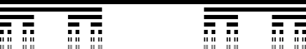
![[0,1]](https://s0.wp.com/latex.php?latex=%5B0%2C1%5D&bg=ffffff&fg=333333&s=0&c=20201002) to a list of two closed intervals:
to a list of two closed intervals: ![[0, 1/3]](https://s0.wp.com/latex.php?latex=%5B0%2C+1%2F3%5D&bg=ffffff&fg=333333&s=0&c=20201002) and
and ![[2/3, 1]](https://s0.wp.com/latex.php?latex=%5B2%2F3%2C+1%5D&bg=ffffff&fg=333333&s=0&c=20201002) .
. 
 is the set of all its subsets. If you’ve ever studied any set theory, this should be familiar. Unfortunately, a typical first course in set theory may not go into the how power sets interact with functions; this is what the “monad” structure of power sets is all about. This structure has three parts, each corresponding to a very common and important mathematical construction, but also so simple enough that we often use it without even thinking about it.
 , there corresponds a function
 , i.e. each subset
  , to its image:
 .
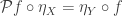
. a functor because the mapping of functions gets along nicely with identity functions and composition. This functor is the first part of the power set monad.
 under
under  , rather than
  . But here, we need to be more careful: despite its frequent use in mathematics,
  is just an extension of
 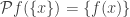 .
. for
for  , as sort of “dual” version of the previous abuse of notation, though I don’t think anyone does that.
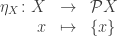
 , which is precisely the equation that makes
  a natural transformation. This natural transformation is the second piece in the monad structure.
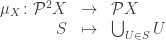
 is the power set of the power set of
  must be compatible in such a way that these diagrams commute:
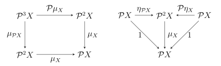

 , but, strictly speaking, this doesn’t parse: we can’t feed a set of triangles into
  , we can’t feed it into
  again doesn’t live in
  —it lives in
  :
:
 we get
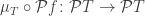
 .
.


 .
. to get the initial state.
 to get a new state, as many times as you want.


 smaller than its parent, where
  is the
 There’s a lot of fascinating structure here, and much of it is directly analogous to the 6-fold and 8-fold cases above, but there are also some differences, stemming from the “cousin rivalry” that goes on in pentagon society.


 And again:
 .
.
 at each step, you’ll get a tessellation of the plane.