Savitzky-Golay filters

There are often two different but equally important descriptions of a given mathematical process — one that makes it simple to calculate and another that makes it simple to understand.

Savitzky-Golay filters are like that. In digital signal processing, they give nice ways to “smooth” a signal, getting rid of small noisy fluctuations while retaining the signal’s overall shape. There are two ways to think about how they work—one based on convolution and another based on approximation by polynomials. It’s not obvious at first why these give the same result, but working out the correspondence is a fun and enlightening exercise.

Graphic by Cdang: Smoothing of noisy data by the Savitzky-Golay method (3^rd degree polynomial, 9 points wide sliding window).

From the name Savitzky-Golay filter, you might well expect one way to think about Savitzky-Golay smoothing is as a convolutional filter.  Indeed, one general method of smoothing a function is to “smear” it with another function, the “filter,” effectively averaging the function’s value at each point with neighboring values.  In this case, the filter function is given by “Savitzky-Golay coefficients.”  You could look these up, or get them from your math software, but they may look rather mysterious until you work out where they came from.  Why these particular coefficients?

The other way to think of Savitzky-Golay smoothing goes as follows.  Suppose you have a digital signal, which for present purposes is just a continuous stream of real numbers:

Now for each , fit a polynomial to on the points between and ,  and replace by the value of this polynomial at .  This approach involves constructing a new polynomial fit at each point: always a polynomial of same degree, but fit to a different set of points.

Again, these two descriptions are equivalent.  The polynomial fit version is a lot more satisfying, in that I can visualize how the smoothing is working, and understand intuitively why this is a good smoothing method.  On the other hand, you wouldn’t want to calculate it using this method, solving a least-squares polynomial fit problem at each step. For calculations, convolution is much faster.

Why are these equivalent?

The key point that makes doing separate least-squares problems at each point equivalent to doing a simple convolution is that we are dealing with digital signals, with values arriving at regularly spaced intervals.  While the dependent variable of the signal could have any crazy behavior you might imagine, the regularity of the independent variable makes most of the least squares calculation the same at each step, and this is what makes the whole process equivalent to a convolution.

Here’s the correspondence in detail.

First, consider how we construct .  This is based on a least squares fit to the points

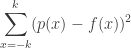
Here’s a quick review of how this works.  The idea is to find coefficients such that this polynomial of degree d:

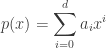
gives the best possible predictions for the values of $f(x)$ in that range.  If , then there will be a polynomial whose graph passes perfectly through all points, but in order to have a smoothing effect, we want .  The problem is then to minimize the total squared error:

We can write this compactly using matrices. First, form the design matrix , a matrix with rows given by

for

For example, if k = 4, and d = 2, will have these entries:

     1   -4   16  -64
     1   -3    9  -27
     1   -2    4   -8
     1   -1    1   -1
     1    0    0    0
     1    1    1    1
     1    2    4    8
     1    3    9   27
     1    4   16   64

Notice that the matrix product , where , then gives a column vector of values for the polynomial :

.

Those are the “predicted” values for , so if we let be the column vector of actual values, then our problem is to find a vector that minimizes

.

The gradient

is zero if and only if the normal equation

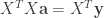
holds.  When is invertible, which is always the case if $d<2k$, this has solution

This gives the coefficients .  Now, what about the value of ?

Our smoothed version of , agrees at 0 with our polynomial approximation .  Since we are evaluating the polynomial at zero, we get just the degree-zero term.  In other words, is just the topmost entry in the above solution.  That is,

where is the first standard basis vector of .

We’re almost done!  Notice that the previous equation just says the value of the smoothed function at is a certain linear combination of the values of in a window of length around 0.

More importantly, if we were to go through the same process to construct for other values of , it is clear that, by a simple shift of coordinates, we would get a linear combination with the same coefficients as above.

And that’s convolution!  The general formula for the smoothing is thus

.

Returning to the example I gave above, with , calculating gives approximately

-0.09091   0.06061   0.16883   0.23377   0.25541   0.23377   0.16883   0.06061  -0.09091
 0.07239  -0.11953  -0.16246  -0.10606   0.00000   0.10606   0.16246   0.11953  -0.07239
 0.03030   0.00758  -0.00866  -0.01840  -0.02165  -0.01840  -0.00866   0.00758   0.03030
-0.01178   0.00589   0.01094   0.00758   0.00000  -0.00758  -0.01094  -0.00589   0.01178

so the Savitzky-Golay filter in this case is just the first row:

-0.09091   0.06061   0.16883   0.23377   0.25541   0.23377   0.16883   0.06061  -0.09091

Convolving any signal with this filter has the effect of replacing the value at each point with the value of the best quadratic polynomial fit to the values at that point and its eight nearest neighbors.